Like flat-earthers, standard statistical models can sometimes be a little detached from reality. If you work in occupational hygiene, you’re likely intimately familiar with the Normal and Lognormal distributions. They are the bread and butter of our industry, but they have a specific quirk that drives me nuts: they allow for “infinite tails.”
Mathematically, this means that standard models suggest there is always a tiny, non-zero probability that an exposure result will reach infinity. Obviously, that’s impossible. You can’t have a concentration of a chemical higher than pure vapour, and you can’t fit more dust into a room than the volume of the room itself. This is where the Beta Distribution steps in to save the day, and it’s why I’ve become such a vocal proponent of its use in our field (#AIOHStatsGang).
The strength of the Beta distribution is that it has hard limits. It allows you to define a minimum and a maximum. By setting a ceiling—an upper bound—we stop the model from predicting unrealistically high results. We are effectively telling the math, “Look, physically, the exposure cannot go higher than X.” This seemingly small change completely removes those phantom probabilities of impossible exposure levels, giving us a statistical picture that actually obeys the laws of physics.

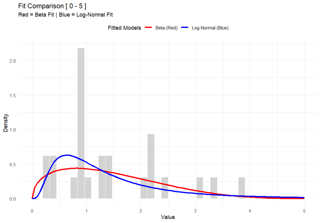
In the chart above (generated using R-base), you can see that while both functions fit the data well, the Beta distribution respects a hard ceiling at 5, whereas the Lognormal tail simply drifts off into the impossible.
But here’s the rub—switching to Beta isn’t for the faint of heart. The Lognormal distribution is easy; you can do it on a napkin with a $5 calculator. The Beta distribution is mathematically more complex and abstract. It’s harder to explain to a layman, and the formulas are heftier. But in my opinion, I’d rather struggle with the math for 10 minutes than present a risk assessment that implies a worker could be exposed to a billion ppm.
This approach also forces us to be better specialists because it brings expert judgement back into the driver’s seat – or at least backseat driving. Because the model relies on fixed boundaries, you can’t just feed it data and walk away. You have to decide where to put those lower and upper bounds based on the specific environment. Today, there are PLENTY of AI tools to help you do this, even in Excel. It forces a deeper engagement with the process conditions rather than blind reliance on a pre-cooked spreadsheet (looking at you IHStat). It might be a headache to set up initially, but a model that respects physical reality is a model worth using.
Further Reading
For a deeper dive into the mathematics of the Beta distribution, check out:
# This work is marked with CC0 1.0.
# To view a copy of this license, visit:
# https://creativecommons.org/publicdomain/zero/1.0/

# Author: Dean Crouch
# Date: 27 January 2026

# Load necessary libraries
if (!require(MASS)) install.packages("MASS")
if (!require(ggplot2)) install.packages("ggplot2")
library(MASS)
library(ggplot2)

# ===========================================================================
# Function: fit_beta_and_lognormal
# (Fits both distributions and plots them with extended axes)
# ===========================================================================
fit_beta_and_lognormal <- function(data, min_val = 0, max_val = 5) {

  # --- 0. VALIDATION CHECK ---
  # Check if any data points fall outside the specified range
  if (any(data < min_val | data > max_val)) {
    message("Error: Data contains values outside the range [", min_val, ", ", max_val, "]. Update your assumed min & max. Exiting function.")
    message(list(data[data < min_val | data > max_val]))
    return(NULL) # Exits the function early
  }

  # --- 1. PREPARE DATA ---
  # Since we validated above, data_clean will be the same as data,
  # but we'll keep the variable name for consistency with your original logic.
  data_clean <- data
  epsilon <- 1e-6 # Nudge for boundaries

  # --- 2. FIT BETA (Red) ---
  # Normalize to [0, 1]
  data_norm <- (data_clean - min_val) / (max_val - min_val)
  data_norm[data_norm <= 0] <- epsilon
  data_norm[data_norm >= 1] <- 1 - epsilon

  fit_beta <- fitdistr(data_norm, "beta", start = list(shape1 = 1, shape2 = 1))
  alpha_est <- fit_beta$estimate["shape1"]
  beta_est <- fit_beta$estimate["shape2"]

  # --- 3. FIT LOG-NORMAL (Blue) ---
  data_lnorm <- data_clean
  data_lnorm[data_lnorm <= 0] <- epsilon

  fit_lnorm <- fitdistr(data_lnorm, "lognormal")
  meanlog_est <- fit_lnorm$estimate["meanlog"]
  sdlog_est <- fit_lnorm$estimate["sdlog"]

  # --- 4. PLOTTING ---
  df <- data.frame(val = data_clean)

  p <- ggplot(df, aes(x = val)) +
    # Histogram
    geom_histogram(aes(y = after_stat(density)), bins = 40, fill = "lightgray", color = "white") +

    # Beta Curve (RED)
    stat_function(fun = function(x) {
      dbeta((x - min_val) / (max_val - min_val), alpha_est, beta_est) / (max_val - min_val)
    }, aes(colour = "Beta (Red)"), linewidth = 1.2) +

    # Log-Normal Curve (BLUE)
    stat_function(fun = function(x) {
      dlnorm(x, meanlog_est, sdlog_est)
    }, aes(colour = "Log-Normal (Blue)"), linewidth = 1.2) +

    # Styling
    scale_x_continuous(limits = c(min_val, max_val)) +
    scale_colour_manual(name = "Fitted Models",
                        values = c("Beta (Red)" = "red", "Log-Normal (Blue)" = "blue")) +
    labs(title = paste("Fit Comparison [", min_val, "-", max_val, "]"),
         subtitle = "Red = Beta Fit | Blue = Log-Normal Fit",
         x = "Value", y = "Density") +
    theme_minimal() +
    theme(legend.position = "top")

  print(p)
}

# ===========================================================================
# Usage Example with BETA Data
# ===========================================================================
set.seed(42)

# 1. Define Range
my_min <- 0
my_max <- 5

# 2. Generate Dummy Data using rbeta (The "True" Source)
# We use shape1=2 and shape2=5, then scale it to 0-5
observed_data <- (rbeta(n = 10, shape1=2, shape2=5) * (my_max - my_min)) + my_min

# 3. Run the Fitting Function
fit_beta_and_lognormal(observed_data, min_val = my_min, max_val = my_max)

Leave a Reply
You must be logged in to post a comment.