Author: Dean

  • IRCP-66 and breathing rates

    Also posted on LinkedIn, but posts on there disapear like smoke in the wind….

    https://lnkd.in/p/gkT8Vbiy

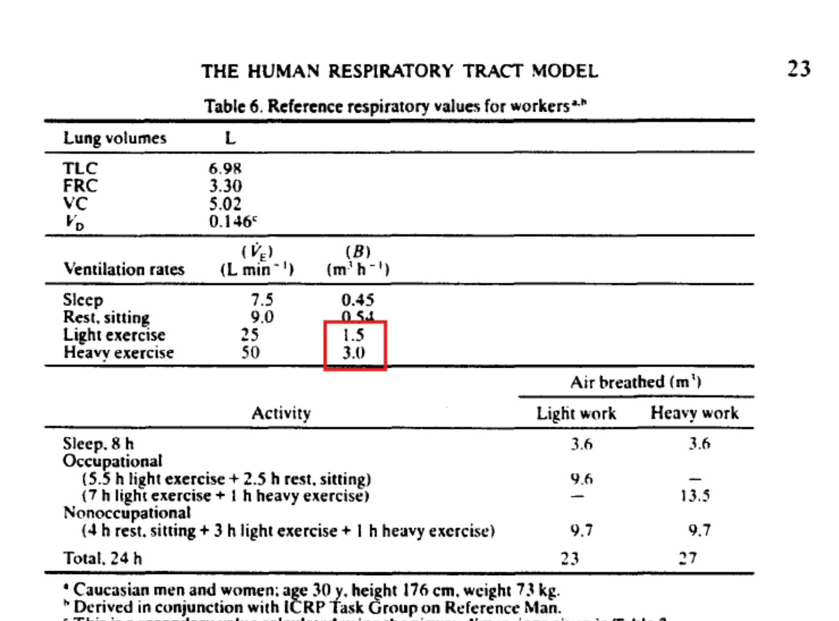
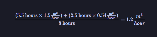
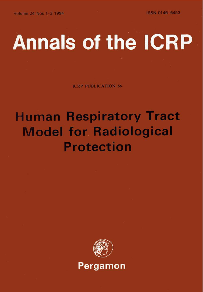
    So you’re minding your own business on a Saturday afternoon, casually reading ICRP-66 on the Human Respiratory Tract Model, and come across Table 6. For those who aren’t ‘initiated’, we generally use the worker breathing rate of 1.2 m3/hr in mining when calculating work category or SEG annual doses from long-lived radioactive dust (LLRD).

    My heart skipped a beat – have I been wrong all this time?

    No, of course not. And shame on you for thinking such a heresy. It turns out workers aren’t going full-tilt for 8 hours – the assumption is 5.5 hours of light exercise at 1.5 m3/hr, then 2.5 hours of sitting around doing SFA at 0.54 m3/hr. We’re not going to discuss the assumption that they never ‘do hard exercise’, a.k.a. work hard.

    Keep the derivation of “1.2 m3/hr” in mind when extending worker shifts to 12 hours, as 5.5 and 2.5 may no longer be valid proportions over 12 instead of 8 hours.

  • Heavy Metal vs Heavy Decay: Why Chemical Analysis Fails for Lead-210

    1. Introduction

    In occupational hygiene and environmental management, lead (Pb) is routinely encountered as an inorganic chemical toxicant. In radiation protection, however, lead also appears as lead-210 (210Pb), a radioactive progeny in the uranium-238 (238U) decay chain commonly present in naturally occurring radioactive material (NORM) scale, mineral sands processing, and dust residues.

    A frequent point of confusion across disciplines is the assumption that analytical techniques used to measure elemental lead concentrations—such as X-ray Fluorescence (XRF) or Inductively Coupled Plasma Mass Spectrometry (ICP-MS)—can be applied to assess 210Pb activity for radiological risk assessment or regulatory exemption.

    I’m going to try and demo, through first-principles specific activity calculations, why standard elemental analysis techniques are completely blind to radiologically significant concentrations of 210Pb, whereas the same techniques remain valid screening tools for primordial radionuclides like 238U and thorium-232 (232Th).

    The fact that sometimes the methods work doesn’t help reduce the confusion but the rule of thumb I’ve just made up is:

    if the half life is long, north of 50 million years, chemistry FTW! If the half life is short, say less than 50 million years you’re going to need to use radio analysis.

    2. Elemental Lead in Occupational Hygiene

    In occupational hygiene, inorganic lead is evaluated as a systemic chemical poison. SafeWork Australia sets the Workplace Exposure Standard (WES) for airborne lead dust and fumes at an eight-hour time-weighted average (TWA) of 0.05 mg/m3, with mandatory biological monitoring based on blood lead concentrations.

    When evaluating bulk materials, surface dust, or air filters for chemical lead hazard characterisation, results are expressed in mass fractions:

    • Parts per million (ppm, or mg/kg)
    • Micrograms per gram (µg/g)
    • Percentage by weight (wt%)

    Typical field and laboratory instrumentation for elemental lead determination includes:

    • Portable X-ray Fluorescence (pXRF): Direct non-destructive measurement with a lower limit of detection (LOD) typically between 5 ppm and 10 ppm for lead.
    • ICP-MS / ICP-OES: Wet-chemical digestion followed by mass or optical emission spectrometry, offering detection limits down to sub-ppm or low parts per billion (ppb) levels.

    These techniques quantify the combined mass of all stable lead isotopes (204Pb, 206Pb, 207Pb, and 208Pb).

    3. Radiation Protection and Lead-210 (210Pb)

    In radiation protection, NORM regulations (such as the ARPANSA Code for Radiation Protection in Planned Exposure Situations, RPS C-1) set the activity concentration exemption and clearance threshold for 210Pb in bulk solid materials at 1 Bq/g (1,000 Bq/kg).

    To determine whether elemental analytical techniques can detect 1 Bq/g of 210Pb, we calculate the physical mass concentration corresponding to this activity concentration using the fundamental decay equation.

    First-Principles Specific Activity Calculation for 210Pb

    The specific activity Asp of a pure radionuclide is derived from its decay constant $\lambda$ and molar mass $M$:

    $$A_{\text{sp}} = \frac{\lambda \cdot N_A}{M} = \frac{\ln(2) \cdot N_A}{T_{1/2} \cdot M}$$

    Where:

    • $N_A = 6.02214 \times 10^{23}\text{ atoms/mol}$ (Avogadro constant)
    • $T_{1/2} = 22.20\text{ years} = 7.007 \times 10^8\text{ s}$ (half-life of 210Pb)
    • $M = 209.984\text{ g/mol}$ (molar mass of 210Pb)

    Calculating the decay constant $\lambda$:

    $$\lambda = \frac{\ln(2)}{7.007 \times 10^8\text{ s}} \approx 9.892 \times 10^{-10}\text{ s}^{-1}$$

    Substituting into the specific activity equation:

    $$A_{\text{sp}} = \frac{(9.892 \times 10^{-10}\text{ s}^{-1}) \cdot (6.02214 \times 10^{23}\text{ atoms/mol})}{209.984\text{ g/mol}} \approx 2.836 \times 10^{12}\text{ Bq/g}$$

    Sidebar: this is the activity of a solid pure gram of Pb-210 and it is a colossal total activity. Not something you want to be handling without a lot of lead shielding; the irony of that statement should be apparent.

    To find the mass fraction $w$ corresponding to an activity concentration of 1 Bq/g:

    $$w = \frac{1\text{ Bq/g}}{A_{\text{sp}}} = \frac{1\text{ Bq/g}}{2.836 \times 10^{12}\text{ Bq/g}} \approx 3.53 \times 10^{-13}\text{ g/g}$$

    Expressed in occupational hygiene concentration units:

    $$w = 0.353\text{ pg/g} = 0.353\text{ parts per trillion (ppt)} = 3.53 \times 10^{-7}\text{ ppm}$$

    Analytical Implications

    A regulatory clearance threshold of 1 Bq/g for 210Pb represents a mass concentration of approximately 0.35 ppt.

    Because standard elemental analytical techniques operate in the ppm or low-ppb range depending on the methodology, chemical techniques are far too insensitive to detect sub-part-per-trillion mass fractions of 210Pb. A sample containing 1 Bq/g of pure 210Pb will be reported by an occupational hygiene laboratory as “Lead: Below Detection Limit”, despite representing a full radiological exemption limit.

    Consequently, 210Pb characterisation requires radiometric methods:

    • Gamma Spectrometry: Measuring the low-energy 46.5 keV gamma transition of 210Pb using planar high-purity germanium (HPGe) detectors.
    • Alpha Spectrometry / Liquid Scintillation: Chemical separation followed by counting the energetic 5.30 MeV alpha emission of its decay progeny, bismuth-210/polonium-210 (210Po), assuming secular equilibrium.

    4. Why Elemental Analysis Works for Uranium and Thorium

    Unlike 210Pb, primordial radionuclides 238U and 232Th have half-lives comparable to the age of the Earth. As a result, their specific activities are vastly lower, making 1 Bq/g correspond to mass fractions that fall well within the detection range of standard chemistry and field pXRF.

    Uranium-238 Calculation

    For 238U:

    • $T_{1/2} = 4.47\text{ billion years} = 1.410 \times 10^{17}\text{ s}$
    • $M = 238.05\text{ g/mol}$

    $$\lambda = \frac{\ln(2)}{1.410 \times 10^{17}\text{ s}} \approx 4.916 \times 10^{-18}\text{ s}^{-1}$$

    $$A_{\text{sp}} = \frac{(4.916 \times 10^{-18}) \cdot (6.02214 \times 10^{23})}{238.05} \approx 12,430\text{ Bq/g} = 12.43\text{ Bq/mg}$$

    The mass fraction $w$ for 1 Bq/g of 238U is:

    $$w = \frac{1\text{ Bq/g}}{12,430\text{ Bq/g}} \approx 8.04 \times 10^{-5}\text{ g/g} = 80.4\text{ ppm}$$

    Because 80.4 ppm exceeds the typical pXRF detection limit (5–10 ppm for uranium) by nearly an order of magnitude, field pXRF elemental readings (ppm U) can be converted directly to activity concentrations (Bq/g U-238) using the factor:

    $$1\text{ Bq/g }^{238}\text{U} \approx 80.4\text{ ppm U} \quad \left(\text{or } 1\text{ ppm U} \approx 0.0124\text{ Bq/g}\right)$$

    Thorium-232 Calculation

    For 232Th:

    • $T_{1/2} = 14.05\text{ billion years} = 4.433 \times 10^{17}\text{ s}$
    • $M = 232.04\text{ g/mol}$

    $$\lambda = \frac{\ln(2)}{4.433 \times 10^{17}\text{ s}} \approx 1.564 \times 10^{-18}\text{ s}^{-1}$$

    $$A_{\text{sp}} = \frac{(1.564 \times 10^{-18}) \cdot (6.02214 \times 10^{23})}{232.04} \approx 4,057\text{ Bq/g} = 4.06\text{ Bq/mg}$$

    The mass fraction $w$ for 1 Bq/g of 232Th is:

    $$w = \frac{1\text{ Bq/g}}{4,057\text{ Bq/g}} \approx 2.46 \times 10^{-4}\text{ g/g} = 246\text{ ppm}$$

    At 246 ppm, 1 Bq/g of 232Th is easily quantified by field pXRF and routine laboratory chemical analysis:

    $$1\text{ Bq/g }^{232}\text{Th} \approx 246\text{ ppm Th} \quad \left(\text{or } 1\text{ ppm Th} \approx 0.00406\text{ Bq/g}\right)$$

    5. Summary Comparison

    The table below contrasts the physical parameters and analytical detection capabilities for 1 Bq/g of key NORM radionuclides, grouped by decay series and ordered by decreasing half-life.

    Radionuclide Half-life (T1/2) Specific Activity (Asp) Mass Fraction for 1 Bq/g Measurable by Field pXRF / ICP-MS? Primary Analytical Method
    Uranium-238 Series
    238U 4.47 billion years 1.24 × 10⁴ Bq/g 80.4 ppm Yes (LOD ≈ 5–10 ppm) Field pXRF, ICP-MS, Gamma Spectrometry
    234U 245,500 years 2.30 × 10⁸ Bq/g 4.34 ppb (0.00434 ppm) No (far below LOD) Alpha Spectrometry, High-Res ICP-MS
    226Ra 1,600 years 3.66 × 10¹⁰ Bq/g 0.027 ppb (0.000027 ppm) No (far below LOD) Gamma Spectrometry (186 keV or 214Pb/214Bi), Radon Emanation
    210Pb 22.20 years 2.84 × 10¹² Bq/g 0.35 ppt (0.00000035 ppm) No (far below LOD) Gamma Spectrometry (46.5 keV), LSC / Alpha Spectrometry
    210Po 138.4 days 1.66 × 10¹⁴ Bq/g 0.006 ppt (0.000000006 ppm) No (far below LOD) Alpha Spectrometry (5.30 MeV) after Spontaneous Deposition
    Thorium-232 Series
    232Th 14.05 billion years 4.06 × 10³ Bq/g 246 ppm Yes (LOD ≈ 5 ppm) Field pXRF, ICP-MS, Gamma Spectrometry
    228Ra 5.75 years 1.01 × 10¹³ Bq/g 0.099 ppt (0.000000099 ppm) No (far below LOD) Gamma Spectrometry (228Ac at 911 keV), Beta Counting

    6. Distinguishing Occupational Hygiene from Radiation Protection

    Understanding the distinct boundary between occupational hygiene and radiation protection is essential for operational safety and regulatory compliance.

    1. Risk Profile and Hazard Mechanism

    • Occupational Hygiene (Chemical Toxicology): Heavy metal lead toxicity depends on systemic chemical uptake (ingestion or inhalation of elemental lead mass), leading to inhibition of haem synthesis, renal impairment, elevated blood lead levels, and neurological effects.
    • Radiation Protection (Ionising Radiation Dose): The hazard from 210Pb arises from ionising radiation delivered to internal tissues. Decay of 210Pb generates beta emissions and gives rise to its short-lived high-energy decay progeny, bismuth-210 (210Bi) and polonium-210 (210Po). Polonium-210 emits a high-LET 5.30 MeV alpha particle, delivering a concentrated committed effective dose to bronchial epithelium upon inhalation.

    2. The Danger of Misinterpreting Units

    Confusing mass concentrations (ppm) with activity concentrations (Bq/g) creates significant operational compliance errors:

    • False Reassurance: Submitting a 210Pb-contaminated scale sample to a standard chemical laboratory will yield a “non-detect” result for lead mass, leading site personnel to mistakenly conclude the material is non-hazardous.
    • Inappropriate Screening: Conversely, using pXRF lead (Pb) readings as an indicator of radiological activity assumes that all lead present is 210Pb. In practice, stable lead isotopes completely dominate the elemental mass, making total lead mass an uninformative metric for radioisotope presence.

    Maintaining clear separation between chemical toxicity metrics (mg/m3, ppm) and radiological activity metrics (Bq/m3, Bq/g) ensures that appropriate sampling protocols, analytical instruments, and risk controls are selected for site characterisation.

  • “Astatine – just say no!” The Thermal Fury of Astatine: Calculating the Heat Output of an element you’ve never heard of.

    This is a follow-on from the very awesome video by Randall Munroe on making a wall made of 1L samples (10x10x10cm) of every element in the periodic table.

    The question is ‘what exactly is the power output of astatine?’


    A solid $7\text{ kg}$ sample of Astatine-210 (the most stable isotope) would generate a thermal output of approximately $233\text{ MW}$ $(233,000,000\text{ watts})$ at the moment of its creation. If the sample consisted of Astatine-211—the isotope commonly created in particle accelerators—the thermal output would climb even higher, reaching roughly $495\text{ MW}$ $^{[1, 2]}$.

    To put this scale into perspective, a 1-litre block of astatine would produce as much heat as a small commercial nuclear reactor, entirely concentrated within a handful of matter.

    But don’t take my word for it; LET’S USE FIRST PRINCIPLES!!!.

    1. Count the Atoms

    To find out how much heat is released, we first determine how many atoms are present in a $7\text{ kg}$ ($7,000\text{ g}$) sample using Avogadro’s number:

    $$N = \frac{\text{Mass}}{\text{Molar Mass}} \times N_A$$

    Using Astatine-210 ($210\text{ g/mol}$) $^{[2]}$:

    $$N = \frac{7,000\text{ g}}{210\text{ g/mol}} \times 6.022 \times 10^{23}\text{ atoms/mol}$$

    $$\approx 2.0073 \times 10^{25}\text{ atoms}$$

    2. Determine the Decay Constant

    Next, we calculate the decay constant ($\lambda$) using the half-life of Astatine-210, which stands at $8.1\text{ hours}$ ($29,160\text{ seconds}$) $^{[3]}$:

    $$\lambda = \frac{\ln(2)}{t_{1/2}} = \frac{0.69315}{29,160\text{ s}}$$

    $$\approx 2.377 \times 10^{-5}\text{ s}^{-1}$$

    3. Calculate Total Radioactivity

    The total radioactivity, or activity ($A$), measured in Becquerels ($\text{Bq}$, decays per second) is the product of the number of atoms and the decay constant:

    $$A = \lambda \times N$$

    $$A = (2.377 \times 10^{-5}\text{ s}^{-1}) \times (2.0073 \times 10^{25})$$

    $$\approx 4.771 \times 10^{20}\text{ Bq}$$

    4. Convert Energy to Watts

    Every individual decay of Astatine-210 releases an average combined radiation energy—comprising alphas, electrons, and photons—of approximately $3.0515\text{ MeV}$. We convert this particle energy into Joules ($1\text{ MeV} = 1.6022 \times 10^{-13}\text{ J}$) $^{[3, 4]}$:

    $$\text{Energy per decay} = 3.0515\text{ MeV} \times 1.6022 \times 10^{-13}\text{ J/MeV}$$

    $$\approx 4.889 \times 10^{-13}\text{ J}$$

    Multiplying the total decays per second by the energy per decay yields the absolute power output:

    $$P = A \times \text{Energy per decay}$$

    $$P = (4.771 \times 10^{20}\text{ Bq}) \times (4.889 \times 10^{-13}\text{ J})$$

    $$\approx 2.333 \times 10^8\text{ W}$$

    5. Final Thermal Output Result

    The hypothetical initial thermal output of a solid $7\text{ kg}$ sample of Astatine-210 sits at $2.33 \times 10^8\text{ watts}$ ($233\text{ MW}$).

    For those who prefer programmatic verification, here is the Python script used to model these calculations based on specific activity and mean energy.

    # Calculate the thermal power of Astatine-210 based on # specific activity and mean energy
    #
    # Specific activity # = 6.817e16 Bq/g
    # Mass = 7000 g
    # Mean energy per decay = 0.0097 + 0.07962 + 2.96215 = # 3.05147 MeV
    
    spec_activity = 6.817e16  # Bq/g
    mass = 7000  # g
    total_activity = spec_activity * mass  # Bq
    
    mean_energy_mev = 3.05147
    energy_j = mean_energy_mev * 1.60218e-13
    
    power_w = total_activity * energy_j
    print(f"At-210 Power: {power_w:.4e} Watts")

    References

    1. Lindegren, S., Albertsson, P., Bäck, T., Jensen, H., Palm, S., & Aneheim, E. (2020). Realizing clinical trials with Astatine-211: The chemistry infrastructure. Cancer Biotherapy and Radiopharmaceuticals, 35(6), 425–436. https://doi.org/10.1089/cbr.2019.3055 Cited by: 114
    2. ChemLin. (2024). Astatine isotopes – list and properties. ChemLin Chemical Elements. https://www.chemlin.org/chemical-elements/astatine-isotopes.php
    3. MIRDSoft. (n.d.). Astatine-210 radionuclide dosimetric data sheet. Medical Internal Radiation Dose (MIRD) Specification Sheets. https://mirdsoft.org/products/MIRDspecs/MIRDspecs_pdfs/At-210.pdf
    4. BenchChem. (2026). An in-depth technical guide to the radiotoxicity and decay products of Astatine-210. BenchChem Technical Guides. https://www.benchchem.com/pdf/An_In_Depth_Technical_Guide_to_the_Radiotoxicity_and_Decay_Products_of_Astatine_210.pdf
  • MCNP and the Hulk

    Knowing how much that software package costs, and this is what they used it for, pleases me greatly 🙂

  • Chi-square tests and romance

    Some while back I had a paper published int he Radiation Protection in Australia journal, the official journal of the Australasian Radiation Protection Society. It was a passion project as at the time no-one could tell me why the pass/fail values for the chi-squared test we did for alpha counting were what they were (ref DMP NORM-3.4).

    So I deep dived it, wrote up the manuscript, got my wife to help and eventually proof read and BAM – we co-authored a paper together.

    #Romance.

    This was actually the first time I realised I could contribute back this way and started a landslide of presnetations, a whole website just so I can drop math-bombs (this website) and other ‘things’.

    Good times 🙂

  • UCL v UTL

    This dataset $[0.1, 0.2, 0.05]$ is the sample set used in Hewett, 2006 so we’re going to use it here too. It perfectly illustrates why the Upper Tolerance Limit (UTL) (the defensive choice for occupational hygiene), and the Upper Confidence Limit (UCL) (serves a different purpose than ‘most exposed worker in a group’) both fail when sample sizes are small.

    To paraphrase multiple regulators I’ve spoken to:

    “We are not as interested in the average exposure to a work group as the potentially highest exposure end of the workgroup exposure distribution”.

    This is where the langauge gets loose and terms are used interchangably; specfically UCL and UTL.

    The Core Difference

    • UCL (of the Mean): Estimates where the average exposure lies, or the limit below which you are confident it sit under.

    NORM.DIST formula: $mean+ 1.645 \times sd$
    NORM.DIST formula: $\bar{x} + 1.645 \times \sigma$

    LOGNORM.DIST: $GM \times GSD^{1.645}$

    • UTL (95/95): Estimates the limit where the worst-case (95th percentile) of the worse-case of exposures of the population – not the sample set- lie with high confidence.

    The $k$-factor for small datasets

    The $k$-factor is a statistical multiplier used to calculate one-sided tolerance limits (like the 95/95 UTL) when the true population mean and standard deviation are unknown. Unlike a standard Z-score—which assumes you have perfect knowledge of the entire population—the $k$-factor explicitly accounts for the sampling error inherent in small datasets. It acts as a “safety margin” or uncertainty penalty: because we are estimating the distribution from only a few data points, $k$ must be significantly larger than a Z-score to ensure we maintain our desired confidence level (e.g., 95%) that a specific proportion of the population is actually covered.

    As the sample size ($n$) increases and our estimate of the population becomes more reliable, the $k$-factor decreases, eventually converging toward the standard normal quantile ($1.645$ for the 95th percentile) as $n$ approaches infinity.


    Comparison of $k$ vs. $z$ (95% Confidence / 95% Coverage)

    Sample Size (n)k-factorZ-score (z0.95​)The “Uncertainty Penalty”
    37.6561.645+365%
    102.9111.645+77%
    302.2201.645+35%
    $\infty$1.6451.6450%

    The Worked Example

    With only three data points, the uncertainty is massive. Even though your “best guess” (point estimate) for the 95th percentile is low, the statistical safety margin required for 95% confidence is huge.

    MetricCalculation LogicResultContext
    Point Estimate (95th %ile)$\exp^{(\bar{y} + 1.645 \cdot s_y)}$0.31“The most likely 95th percentile.”
    UCL95 (of the Mean)Land’s H-statistic calculation~2.8“We are 95% sure the average is below 2.8.”
    UTL 95/95$\exp^{(\bar{y} + 7.656 \cdot s_y)}$20.2“We are 95% sure 95% of shifts are below 20.2.”

    How to Calculate It

    The “jump” from 0.31 to 20.2 happens because of the $k$-factor, which penalizes the small sample size ($n=3$).

    Log-Transform the data

    $\ln(0.05) = -3.0$,

    $\ln(0.1) = -2.3$,

    $\ln(0.2) = -1.6$

    Descriptive statistics

    $\bar{y} = -2.3$, $GM = 1.0$

    $s_y = 0.693$, $GSD = 2.00$

    Select the K-Factor

    Account for n=3. For a 95/95 limit with 3 samples, use $k = 7.656$. (For $n=20$, this would drop to ~2.4).

    Calculate the Limit

    $UTL = \exp^{(-2.3 + (7.656 \cdot 0.693))} = \exp^{(3.0)} \approx \mathbf{20.2}$.


    The “Sample Size Penalty” Simulator

    You can use this tool to see how increasing your sample size ($n$) collapses the massive gap between your point estimate (0.31) and your defensible 95/95 limit (20.2).

    The 95/95 Tolerance Simulator

    This tool demonstrates the difference between a Point Estimate (a best guess) and the 95/95 UTL (the defensible compliance limit). As sample size increases, the gap between these two numbers narrows.

    Small sets carry a high “uncertainty penalty.”

    Calculated Exposure Limits

    Point Estimate (95th %ile) 0.31
    95/95 Upper Tolerance Limit 20.2
    The red bar shows the “Defensible Limit.”

    UCL (Upper Confidence Limit): Used for long-term averages. For the set above, the UCL of the mean is ~2.8. It is lower than the UTL because it measures the group average, not individual extreme shifts.

    UTL (Upper Tolerance Limit): This is the 95/95 limit. With only 3 samples, the UTL of 20.2 is roughly 65 times higher than the point estimate. By increasing your sample size to 20, you’ll see the UTL “penalty” drop dramatically.

  • Sample quotas all up in this place

    Sample quotas all up in this place

    Catching the Risk: The Maths Behind Sample Quotas in SEGs

    In occupational hygiene, we often talk about Similar Exposure Groups (SEGs) and the need to collect enough samples to be confident in our data. But how do we actually determine if our sample size is sufficient to capture those at the highest risk?

    Standard practice is to mornally just quote Technical Appendix A in NIOSH 173/77 and go from there – but this time, that just wasn’t going to be enough.

    During a recent mentoring session, we broke down the statistics of sampling quotas. Here is how the maths of permutations and combinations helps us ensure no worker is left behind.

    The Foundation: Factorials and Choices

    Before we can calculate the probability of a successful sampling campaign, we need to understand how many ways we can “choose” workers from a group.

    Factorials

    The factorial ($n!$) is the product of all positive integers less than or equal to $n$. This value represents the total number of ways you can uniquely arrange a set of items. For example, if you have 6 items and want to know every possible sequence they could be ordered in:

    $$6! = 6 \times 5 \times 4 \times 3 \times 2 \times 1 = \mathbf{720 \text{ ways to arrange 6 items}}$$

    Permutations vs. Combinations

    Understanding the difference between these two is critical for sampling.

    Permutations

    How many ways can I choose $r$ things from $n$ things where order is important? To use our example of 6 items, let’s say I want to select 2. I can do that by:

    $$6 \times 5 = 30$$

    To get that, using only factorials, we can use some numerator/denominator cancellation. It looks like this, noting how $4 \times 3 \times 2 \times 1$ appears in both the top and bottom and so cancel out:

    $$^nP_r = \frac{6!}{(6-2)!} = \frac{6!}{4!} = \frac{6 \times 5 \times 4 \times 3 \times 2 \times 1}{4 \times 3 \times 2 \times 1} = 6 \times 5 = 30$$

    MAGIC!

    The general formula is:

    $$^nP_r = \frac{n!}{(n-r)!}$$

    Combinations

    How many ways can I choose $r$ things from $n$ things where order is NOT important? In our example of 30 permutations of 2 items, we divide by the 2 ways those items can be arranged ($2 \times 1 = 2$). So let’s divide our permutation formula by the factorial of $r$:

    $$\frac{6!}{2! \times (6-2!)} = \frac{6 \times 5 \times 4 \times 3 \times 2 \times 1}{(2 \times 1)(4 \times 3 \times 2 \times 1)} = \frac{6 \times 5}{2} = 15$$

    $$^n\mathcal{C}_r = \frac{n!}{r! \times (n-r)!}$$

    Practical Example: Choosing 3 Workers from 10

    To see why this distinction matters, imagine you have a group of 10 workers ($n=10$) and you want to select 3 ($r=3$) for monitoring.

    The Permutation Approach (Order Matters)

    If we cared about the order (e.g., who gets the pump first, second, and third), the maths looks like this:

    $$^{10}P_3 = \frac{10!}{(10-3)!} = \frac{10!}{7!} = 10 \times 9 \times 8 = \mathbf{720 \text{ ways}}$$

    The Combination Approach (Order Does Not Matter)

    In a typical hygiene survey, we don’t care about the sequence—only the final set of people monitored. We divide the permutations by the ways those 3 people can be rearranged ($3!$):

    $$^{10}\mathcal{C}_3 = \frac{720}{3 \times 2 \times 1} = \frac{720}{6} = \mathbf{120 \text{ ways}}$$

    Why this matters: There are far fewer unique “groups” than “orders.” We use combinations because we are looking for the probability of a specific subset of the population being captured but what order we select them is not important.

    Defining the Sampling Problem

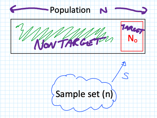
    When sampling a population ($N$), we are often looking for a specific “Target” group ($N_0$), such as a Highly Exposed Risk Group (e.g., the top 10% of exposed workers).

    The critical question is: What is the probability that I get ZERO samples from my high-risk group?

    To find this, we look at the three components of the probability calculation:

    Combinations of $n$ samples from the non-target group $(N – N_0)$.

    Combinations of 0 samples from the target group $(N_0)$.

    Total possible combinations of $n$ samples from the entire population ($N$).

    The maths behind this derivation follows a logical flow:

    $$P(r=0) = \frac{^{(N-N_0)}\mathcal{C}_n \times ^{N_0}\mathcal{C}_0}{^N\mathcal{C}_n}$$

    Since any combination of 0 items ($^{N_0}\mathcal{C}_0$) is equal to 1 (there is only 1 way to select nothing; it makes maths-sense, go with it), we expand the factorials as follows:

    $$P(r=0) = \frac{(N-N_0)!}{n!(N-N_0-n)!} \times \frac{N_0!}{0!(N_0-0)!} \times \left[ \frac{N!}{n!(N-n)!} \right]^{-1}$$

    By simplifying the expressions (flipping the $^N\mathcal{C}_n$ with a $-1$ power) and cancelling out terms (specifically $n!$), we arrive at the final simplified formula:

    $$P(r=0) = \frac{(N-N_0)!}{(N-N_0-n)!} \times \frac{(N-n)!}{N!}$$

    Case Study: Sampling a Population of 18

    Let’s apply this to a group of 18 workers ($N=18$). We want to ensure we haven’t missed the top 10% of exposed workers ($18 \times 0.1 = 1.8$, which we call 2 workers, so $N_0 = 2$).

    If we collect different sample sizes ($n$), how does your risk of “missing” ($r=0$) that high-risk group change?

    Scenario A: Collect 9 Samples ($n=9$)

    Using our formula $\frac{(N-N_0)!}{(N-N_0-n)!} \times \frac{(N-n)!}{N!}$:

    $$P(r=0) = \frac{(18-2)!}{(18-2-9)!} \times \frac{(18-9)!}{18!} = \frac{16!}{7!} \times \frac{9!}{18!} = \mathbf{0.235}$$

    With 9 samples, there is a 23.5% chance you will not capture a single person from that top 10% high-risk group.

    Scenario B: Collect 12 Samples ($n=12$)

    $$P(r=0) = \frac{(18-2)!}{(18-2-12)!} \times \frac{(18-12)!}{18!} = \frac{16!}{4!} \times \frac{6!}{18!} = \mathbf{0.098}$$

    By increasing to 12 samples, your risk of missing the high-risk group drops to roughly 9.8%.

    Scenario C: Collect 15 Samples ($n=15$)

    $$P(r=0) = \frac{(18-2)!}{(18-2-15)!} \times \frac{(18-15)!}{18!} = \frac{16!}{1!} \times \frac{3!}{18!} = \mathbf{0.0196}$$

    At 15 samples, the probability of missing the target group is less than 2%, providing a very high level of certainty.

    The “Flip It” Rule

    In hygiene, we usually want to know the confidence level—the probability of getting at least one sample from the target group ($r \ge 1$). To find this, simply “flip” the result:

    $$\text{Confidence} = 1 – P(r=0)$$

    With 12 samples, you have a 90.2% confidence level

    i.e. $(1-0.098) \times 100$.

    With 15 samples, you have a 98.04% confidence level 

    i.e. $(1-0.0196) \times 100$.

    By using these calculations, you can move away from “guessing” your sample quotas and start providing a statistical justification for your monitoring programs.

    BONUS: And I made a calculator for you!!

    Sample Quota calculator

  • The Web revival

    A very good explanation why I chose to start a personal professional website, and create content here, instead of handing my ideas over to the social media platforms.

    And yes, I had to learn a LOT to get this up and running and it was very satisfying.

  • Contamination & ‘de minimis’

    “Contaminated” isn’t a binary state. It’s the start of a conversation, not the end of one.

    In the world of radiation protection, there is a common reflex to treat “contamination” as a hard “No” for the release of items or materials. If it’s contaminated, it stays in the controlled zone. Simple, right?

    Actually, no. You’re making the solution harder by making the problem easier.

    The term “contamination” describes the presence of radioactive substances. It does not automatically define the risk, nor does it dictate a permanent restriction from the public domain. When we look at primary sources like IAEA-TECDOC-855, the logic is clear: we manage risk, not just atoms.

    The IAEA framework for unconditional clearance is built on the principle of “triviality”—specifically, ensuring that the individual dose to a member of the public remains below ~10 µSv/year.

    To achieve this, the IAEA doesn’t just guess; they categorise radionuclides across five orders of magnitude based on their hazard profile:

    • High Hazard (0.3 Bq/g): For nuclides like Co-60, Ra-226, and Pu-239, the clearance levels are appropriately conservative.
    • Moderate Hazard (30 Bq/g): Common isotopes like C-14 or P-32 have thresholds 100x higher than alpha emitters.
    • Low Hazard (3,000 Bq/g): For H-3 (Tritium) or Ni-63, the “trivial” threshold is ten thousand times higher than for Plutonium.

    Key takeaways for RSOs and regulators:

    1. Nuclide-Specific Nuance: Finding “contamination” on a Surface Contaminated Object (SCO) is just the trigger. The identity of the isotope changes the “acceptable” level by a factor of 10,000.
    2. The Sum of Ratios: For mixtures, we don’t just look at the highest peak. We apply the rigorous formula to ensure the total impact remains trivial.
      ∑CiCLi≤1\sum \frac{C_i}{CL_i} \leq 1
    3. Surface vs. Bulk: In the absence of specific surface guidance, the TECDOC suggests that these same numerical values (Bq/g) can often be applied as surface contamination limits (Bq/cm2) for unconditional release.

    We need to move past the “zero-tolerance” myth and lean back into the science of clearance. The definition of contamination identifies the presence; the science of clearance determines the future.

    Let’s stop asking “Is it contaminated?” and start asking “What is the actual risk, and how do we optimise the outcome?”

    References

    IAEA (1996). Clearance levels for radionuclides in solid materials: Application of exemption principles. Interim report for comment. IAEA-TECDOC-855. Vienna.

  • Here comes the Beta distribution!!!

    Like flat-earthers, standard statistical models can sometimes be a little detached from reality. If you work in occupational hygiene, you’re likely intimately familiar with the Normal and Lognormal distributions. They are the bread and butter of our industry, but they have a specific quirk that drives me nuts: they allow for “infinite tails.”

    Mathematically, this means that standard models suggest there is always a tiny, non-zero probability that an exposure result will reach infinity. Obviously, that’s impossible. You can’t have a concentration of a chemical higher than pure vapour, and you can’t fit more dust into a room than the volume of the room itself. This is where the Beta Distribution steps in to save the day, and it’s why I’ve become such a vocal proponent of its use in our field (#AIOHStatsGang).

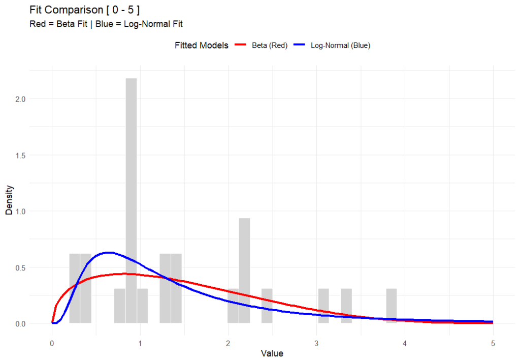
    The strength of the Beta distribution is that it has hard limits. It allows you to define a minimum and a maximum. By setting a ceiling—an upper bound—we stop the model from predicting unrealistically high results. We are effectively telling the math, “Look, physically, the exposure cannot go higher than X.” This seemingly small change completely removes those phantom probabilities of impossible exposure levels, giving us a statistical picture that actually obeys the laws of physics.

    In the chart above (generated using R-base), you can see that while both functions fit the data well, the Beta distribution respects a hard ceiling at 5, whereas the Lognormal tail simply drifts off into the impossible.

    But here’s the rub—switching to Beta isn’t for the faint of heart. The Lognormal distribution is easy; you can do it on a napkin with a $5 calculator. The Beta distribution is mathematically more complex and abstract. It’s harder to explain to a layman, and the formulas are heftier. But in my opinion, I’d rather struggle with the math for 10 minutes than present a risk assessment that implies a worker could be exposed to a billion ppm.

    This approach also forces us to be better specialists because it brings expert judgement back into the driver’s seat – or at least backseat driving. Because the model relies on fixed boundaries, you can’t just feed it data and walk away. You have to decide where to put those lower and upper bounds based on the specific environment. Today, there are PLENTY of AI tools to help you do this, even in Excel. It forces a deeper engagement with the process conditions rather than blind reliance on a pre-cooked spreadsheet (looking at you IHStat). It might be a headache to set up initially, but a model that respects physical reality is a model worth using.


    Further Reading

    For a deeper dive into the mathematics of the Beta distribution, check out:


    # This work is marked with CC0 1.0. 
    # To view a copy of this license, visit:
    # https://creativecommons.org/publicdomain/zero/1.0/
    
    # Author: Dean Crouch
    # Date: 27 January 2026
    
    # Load necessary libraries
    if (!require(MASS)) install.packages("MASS")
    if (!require(ggplot2)) install.packages("ggplot2")
    library(MASS)
    library(ggplot2)
    
    # ===========================================================================
    # Function: fit_beta_and_lognormal
    # (Fits both distributions and plots them with extended axes)
    # ===========================================================================
    fit_beta_and_lognormal <- function(data, min_val = 0, max_val = 5) {
      
      # --- 0. VALIDATION CHECK ---
      # Check if any data points fall outside the specified range
      if (any(data < min_val | data > max_val)) {
        message("Error: Data contains values outside the range [", min_val, ", ", max_val, "]. Update your assumed min & max. Exiting function.")
        message(list(data[data < min_val | data > max_val]))
        return(NULL) # Exits the function early
      }
      
      # --- 1. PREPARE DATA ---
      # Since we validated above, data_clean will be the same as data, 
      # but we'll keep the variable name for consistency with your original logic.
      data_clean <- data 
      epsilon <- 1e-6 # Nudge for boundaries
      
      # --- 2. FIT BETA (Red) ---
      # Normalize to [0, 1]
      data_norm <- (data_clean - min_val) / (max_val - min_val)
      data_norm[data_norm <= 0] <- epsilon
      data_norm[data_norm >= 1] <- 1 - epsilon
      
      fit_beta <- fitdistr(data_norm, "beta", start = list(shape1 = 1, shape2 = 1))
      alpha_est <- fit_beta$estimate["shape1"]
      beta_est <- fit_beta$estimate["shape2"]
      
      # --- 3. FIT LOG-NORMAL (Blue) ---
      data_lnorm <- data_clean
      data_lnorm[data_lnorm <= 0] <- epsilon 
      
      fit_lnorm <- fitdistr(data_lnorm, "lognormal")
      meanlog_est <- fit_lnorm$estimate["meanlog"]
      sdlog_est <- fit_lnorm$estimate["sdlog"]
      
      # --- 4. PLOTTING ---
      df <- data.frame(val = data_clean)
      
      p <- ggplot(df, aes(x = val)) +
        # Histogram
        geom_histogram(aes(y = after_stat(density)), bins = 40, fill = "lightgray", color = "white") +
        
        # Beta Curve (RED)
        stat_function(fun = function(x) {
          dbeta((x - min_val) / (max_val - min_val), alpha_est, beta_est) / (max_val - min_val)
        }, aes(colour = "Beta (Red)"), linewidth = 1.2) +
        
        # Log-Normal Curve (BLUE)
        stat_function(fun = function(x) {
          dlnorm(x, meanlog_est, sdlog_est)
        }, aes(colour = "Log-Normal (Blue)"), linewidth = 1.2) +
        
        # Styling
        scale_x_continuous(limits = c(min_val, max_val)) +
        scale_colour_manual(name = "Fitted Models", 
                            values = c("Beta (Red)" = "red", "Log-Normal (Blue)" = "blue")) +
        labs(title = paste("Fit Comparison [", min_val, "-", max_val, "]"),
             subtitle = "Red = Beta Fit | Blue = Log-Normal Fit",
             x = "Value", y = "Density") +
        theme_minimal() +
        theme(legend.position = "top")
      
      print(p)
    }
    
    # ===========================================================================
    # Usage Example with BETA Data
    # ===========================================================================
    set.seed(42)
    
    # 1. Define Range
    my_min <- 0
    my_max <- 5
    
    # 2. Generate Dummy Data using rbeta (The "True" Source)
    # We use shape1=2 and shape2=5, then scale it to 0-5
    observed_data <- (rbeta(n = 10, shape1=2, shape2=5) * (my_max - my_min)) + my_min
    
    # 3. Run the Fitting Function
    fit_beta_and_lognormal(observed_data, min_val = my_min, max_val = my_max)